14 sorting algorithms in just 60 seconds
14 Sorting Algorithms Explained in 60 Seconds (Quick-Fire Guide)
Need to understand sorting algorithms fast? We break down 14 critical methods used in computer science—each with its strengths, quirks, and ideal use cases—in just 60 seconds. Let’s race!
1. Bubble Sort
How it works: Compares adjacent elements, swapping them if out of order.
Time complexity: O(n²) worst/average case.
Use case: Tiny datasets, educational purposes.
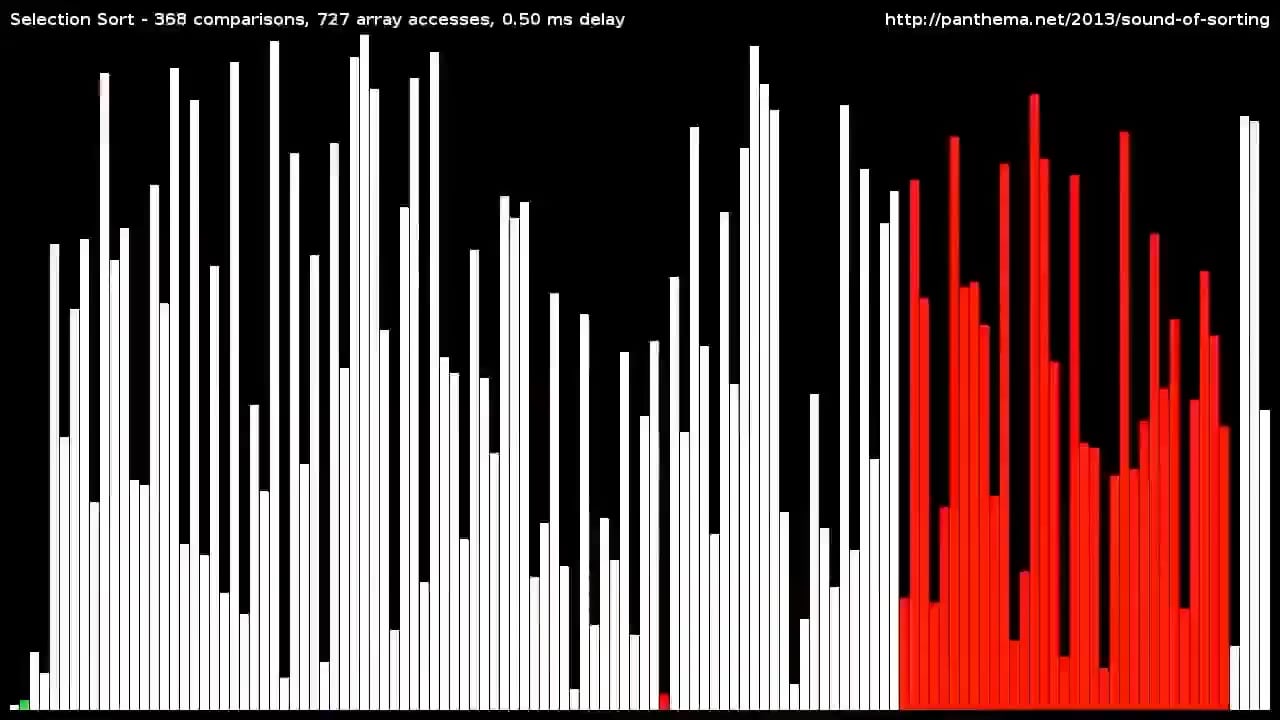
2. Selection Sort
How it works: Finds the smallest element, swaps it to the front. Repeats.
Time complexity: O(n²).
Use case: Small lists, minimal memory usage.
3. Insertion Sort
How it works: Builds a sorted sublist by inserting elements one by one.
Time complexity: O(n²) average, O(n) best (if nearly sorted).
Use case: Small/partially sorted data (e.g., live streaming inputs).
4. Merge Sort
How it works: “Divide and conquer” splits data, sorts, then merges sublists.
Time complexity: O(n log n) for all cases.
Use case: Large datasets, external sorting (stable and efficient).
5. Quick Sort
How it works: Picks a “pivot,” partitions data around it, recurses.
Time complexity: O(n log n) average, O(n²) worst (rare).
Use case: General-purpose, fastest for average cases.
6. Heap Sort
How it works: Converts data into a heap structure, extracts max/min elements.
Time complexity: O(n log n).
Use case: When worst-case performance matters more than average-case.
7. Counting Sort
How it works: Tracks element frequencies, calculates positions.
Time complexity: O(n + k) (k = range of values).
Use case: Small integer ranges (e.g., grades 1–100).
8. Radix Sort
How it works: Sorts digit by digit (LSD or MSD).
Time complexity: O(nk) (k = max digit count).
Use case: Large numbers or strings (phone numbers, dictionaries).
9. Bucket Sort
How it works: Splits data into “buckets,” sorts each individually.
Time complexity: O(n²) worst, O(n+k) average.
Use case: Uniformly distributed data (e.g., 0–1 floats).
10. Shell Sort
How it works: Improved insertion sort with gap sequences.
Time complexity: O(n log n) to O(n²) (depends on gaps).
Use case: Mid-sized datasets with low overhead.
11. Tim Sort
How it works: Hybrid of merge sort + insertion sort (used in Python, Java).
Time complexity: O(n log n).
Use case: Real-world data (optimized for pre-sorted chunks).
12. Comb Sort
How it works: Bubble sort variant with shrinking gaps.
Time complexity: O(n²) worst, O(n log n) average.
Use case: Simple alternative to Shell sort.
13. Cycle Sort
How it works: Minimizes writes by cycling elements to correct positions.
Time complexity: O(n²)
Use case: Memory-constrained systems (e.g., flash memory).
14. Bogo Sort
How it works: Randomizes data until sorted (yes, really).
Time complexity: O(∞) worst, O(n!) average.
Use case: Academic novelty—never in production!
Key Takeaways in 5 Seconds 🚀
- Need speed? Quick Sort or Merge Sort for large sets.
- Memory-sensitive? Heap Sort or Cycle Sort.
- Small data? Insertion/Bubble/Selection Sort.
- Specialized data? Radix, Counting, or Bucket Sort.
Remember: Big O isn’t everything! Stability, memory, and data patterns matter too. Master these, and you’ll sort any challenge efficiently!
(Time’s up! ⏱️)